Compressed vector Prony analysis
for supercritical Hopf bifurcation
in computational fluid dynamics

G. D. McBain

J. A. Edwards (UNSW)

S. G. Mallinson (Memjet, UNSW)

65th Annual Meeting of the Australian Mathematical Society

Thur. 9 December 2021, Newcastle

Supercritical Hopf bifurcation

• Unsteady Navier–Stokes solutions by scikit-fem (Gustafsson & GDMcB 2020)

Point-probe vorticity in near wake

$$\mathrm e^{st} = \mathrm e^{\sigma t} \mathrm e^{\mathrm i\omega t},\qquad |\sigma| \ll \omega$$

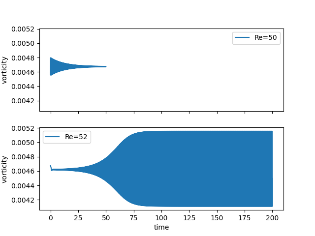
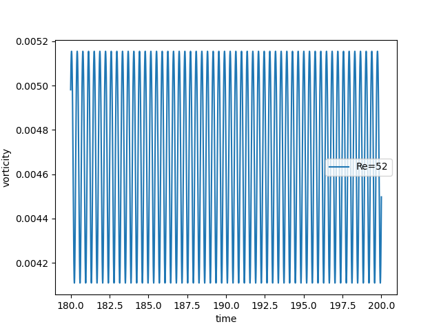
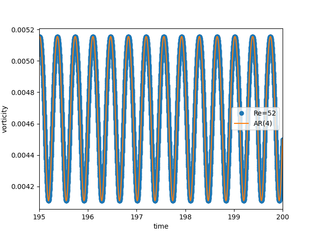
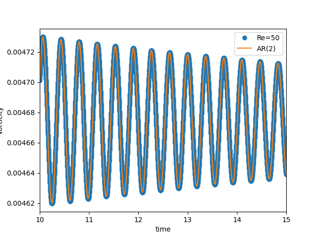
Point-probes: the supercritical periodic oscillations

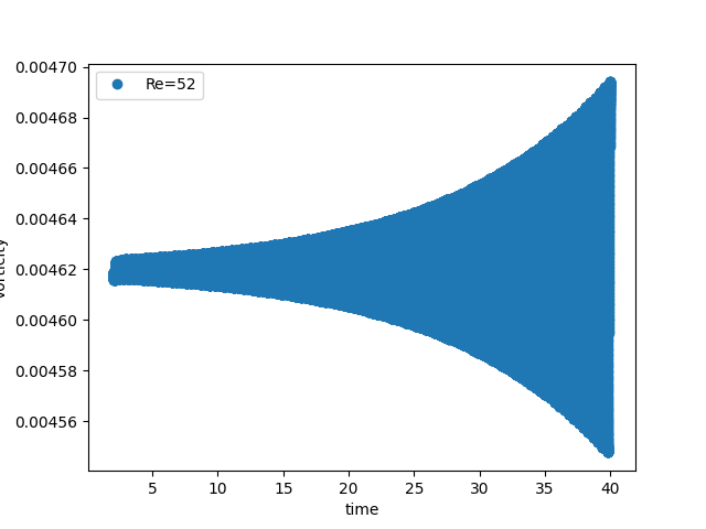
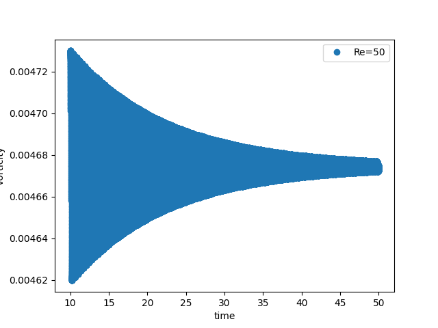
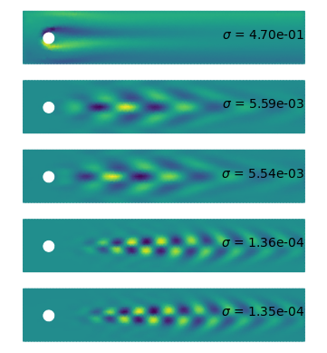
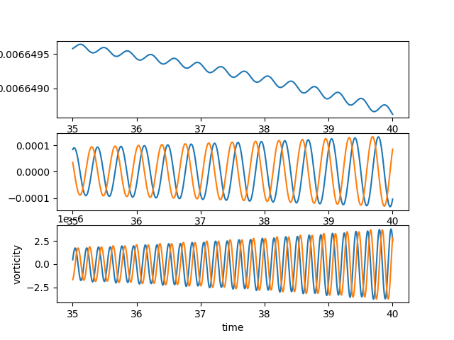
Point-probes: exponential growth from equilibrium

Point-probes: exponential decay to equilibrium

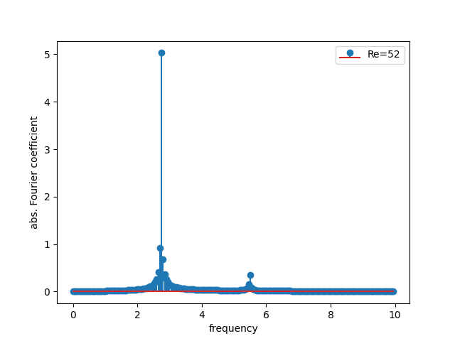
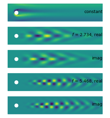
Periodic point-probes: Fourier analysis?

Periodic point-probes: autoregression

• AR(p): $y_k = b_0 + b_1 y_{k-1} + b_2 y_{k-2} + \cdots + b_p y_{k-p}$
  • solve for coefficients by least-squares
• constant term: $y_\infty = b_0 / \left(1 - b_1 - b_2 - \cdots - b_p\right)$
• modes: $y_k - y_\infty \sim a\mu^k$
• characteristic polynomial: $b_p + b_{p-1} \mu + \cdots + b_1\mu^{p-1} - \mu^p$
• complex growth-rate: $s = \left(\log \mu\right) / \Delta t$
• growth rate and angular frequency: $s = \sigma + \mathrm i\omega$

Periodic point-probes: AR v. FFT

• FFT
  • frequency is discretized ± 0.05!
    • 0.05 = 1/20 = 1/duration
  • frequency–time uncertainty: energy is smeared out
  • f = 2.75, 5.50, …
• AR(4):
  • best frequency estimates, not discretized
  • a Prony coefficient contains all the energy of each mode
  • f = 2.742, 5.486, …

AR(p) for periodic point-probes

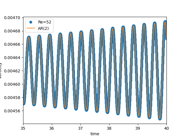
Periodic point-probes: AR for linear growth

• Near the bifurcation point we expect behaviour like $\mathrm e^{st} = \mathrm e^{\sigma t}\mathrm e^{\mathrm i\omega t}$ with |σ| ≪ ω
• This too is just as amenable to autoregression
• FFT is useless
• AR gives both growth rate and frequency:
  • real and imaginary parts of roots of characteristic equation

AR(p) for unstable point-probes

AR(p) for stable point-probes

Fourier v. Prony analysis

• Fourier analysis: series of trigonometric polynomials or complex exponentials of unit modulus

$$y_k = a_0 + a_1 \mathrm e^{\mathrm ik\omega \Delta t} + a_2 \mathrm e^{2\mathrm ik\omega \Delta t} + \cdots + \mathrm{c.c.}$$

• Prony analysis: series of general complex exponentials $\mu = \mathrm e^{s\Delta t}, s = \sigma + \mathrm i\omega$

$$y_k = y_\infty + a_1 \mu_1^k + a_2 \mu_2^k + \cdots + a_p \mu_p^k$$

• Prony, R. (1795). Essai Experimental et Analytique sur les lois de la Dilatabilité de fluides élastiques et sur celles de la Force expansive de la vapeur de l'eau et de l'alkool, à différentes températures. Journal de l'école polytechnique, 1:24–76.

Prony analysis

Three steps:

1. autoregression: $\{y_k\}\rightarrow \{b_\ell\}$, least squares $$y_k = b_0 + b_1 y_{k-1} + b_2 y_{k-2} + \cdots + b_p y_{k-p}$$
2. eigenvalues: $\{b_\ell\}\rightarrow \{\mu_m\}$, roots of characteristic AR polynomial $$b_p + b_{p-1}\mu + \cdots + b_1 \mu^{p-1} - \mu^p$$
3. Prony coefficients: $\left(\{y_k\}, \{\mu_m\}\right)\rightarrow \{a_n\}$, least squares, again $$y_k = y_\infty + a_1 \mu_1^k + a_2 \mu_2^k + \cdots + a_p \mu_p^k$$

Vector Prony Analysis

What if we wanted to apply this to more than just a point-probe?

1. AR → VAR
2. roots of characteristic polynomial → polynomial eigenvalue problem
3. coefficients → still least squares, just bigger

Vector Prony Analysis, 1: VAR(p)

• Vector autogression (VAR(p)) is well established, particularly in econometrics.
  • AR: $y_k = b_0 + b_1 y_{k-1} + b_2 y_{k-2} + \cdots + b_p y_{k-p}$
  • VAR: $\mathbf y_k = \mathbf b_0 + \mathsf B_1 \mathbf y_{k-1} + \mathsf B_2 \mathbf y_{k-2} + \cdots + \mathsf B_p \mathbf y_{k-p}$
• Used to investigate time-series which may be interdependent.
• Straightforward.
• Many implementations available
  • e.g. statsmodels.tsa.vector_ar in Python
• References:
  • Lütkepohl, H. (1991). Introduction to multiple time series analysis., Springer
  • Wikipedia, ‘Vector autoregression’

Vector Prony Analysis, 2(a): PEP, derivation

• characteristic polynomial of AR: substitute $y_k - y_\infty = \mu^k$ into AR's homogenized recurrence relation
  • $b_p + b_{p-1}\mu + \cdots + b_1 \mu^{p-1} - \mu^p$

• Generalization to VAR?

• First find fixed-point of recurrence relation:

$$\begin{align*} \mathbf y_\infty &= \mathbf b_0 + \left(\mathsf B_1 + \mathsf B_2 + \cdots + \mathsf B_p\right) \mathbf y_\infty \\ &= \left(\mathsf I - \mathsf B_1 - \mathsf B_2 - \cdots - \mathsf B_p\right)^{-1} \mathbf b_0 \end{align*}$$

• Then subtract it to homogenize: $\mathbf z_k = \mathbf y_k - \mathbf y_\infty$ $$\mathbf z_k = \mathsf B_1 \mathbf z_{k-1} + \mathsf B_2 \mathbf z_{k-2} + \cdots + \mathsf B_p \mathbf z_{k-p}.$$
• Try $\mathbf z_k = \mu^k\mathbf u$: $$\left[\mathsf B_p + \mu\mathsf B_{p-1} + \cdots + \mu^{p-1}\mathsf B_1\right]\mathbf u = \mu^p\mathbf u$$
• a Polynomial Eigenvalue Problem (PEP)

Vector Prony Analysis, 2(b): PEP, solution

$$\left[\mathsf B_p + \mu\mathsf B_{p-1} + \cdots + \mu^{p-1}\mathsf B_1\right]\mathbf u = \mu^p\mathbf u$$

• Typically convert to standard eigenvale problem $\mu\mathbf v = \mathsf C\mathbf v$ via companion matrix C:

$$ \mu\mathbf v = \mathsf C \mathbf v \equiv \begin{bmatrix} \mathsf B_1 & \mathsf B_2 & \cdots & & \mathsf B_p \\ \mathsf I & 0 & \\ 0 & \mathsf I \\ & & \ddots \\ & & & \mathsf I & 0 \end{bmatrix} \begin{bmatrix} \mu^{p-1}\mathbf u \\ \mu^{p-2}\mathbf u \\ \mu^{p-3}\mathbf u \\ \vdots \\ \mathbf u \end{bmatrix} $$

Vector Prony Analysis, 3: LS

• Vector Prony: $$\mathbf y_k = \mathbf y_\infty \sum_\ell a_\ell \mu_\ell^k \mathbf u_\ell$$
  • ‘dynamic modes’ u_*ℓ*
  • VAR/(HO)DMD eigenvalues μ_ℓ
  • Prony coefficients a_ℓ
• Determine vector Prony coefficients a_ℓ by least squares.

$$\begin{align*} \sum_\ell \mathbf u_\ell \mu_\ell^k a_\ell &= \mathbf y_k - \mathbf y_\infty\,,\qquad (k = 0, 1, \ldots) \\ \begin{bmatrix} \mathsf U \\ \mathsf U\;\mathrm{diag}\mu \\ \vdots \\ \mathsf U\;\mathrm{diag}\mu^{m-1} \end{bmatrix} \begin{bmatrix} a_0 \\ a_1 \\ \vdots\\ a_{pr-1} \end{bmatrix} &= \begin{bmatrix} \mathbf y_0 - \mathbf y_\infty \\ \mathbf y_1 - \mathbf y_\infty \\ \vdots \\ \mathbf y_{m-1} - \mathbf y_\infty \end{bmatrix} \end{align*} $$

Dynamic mode decomposition

• Schmid, P. J. (2010). Dynamic mode decomposition of numerical and experimental data. J. Fluid Mech., 656:5–28

$$\mathbf y_k = \mathsf B \mathbf y_{k-1}$$

• DMD is vector autoregression VAR(1) without constant term!

Higher order dynamic mode decomposition

• Le Clainche, S. & Vega, J. M. 2017. Higher order dynamic mode decomposition. SIAM Journal on Applied Dynamical Systems, 16:882–925
• Vega, J. M., Le Clainche, S. 2020. Higher Order Dynamic Mode Decomposition and its Applications. Academic

$$\mathbf y_k = \mathsf B_1 \mathbf y_{k-1} + \mathsf B_2 \mathbf y_{k-2} + \cdots + \mathsf B_p \mathbf y_{k-p}$$

• Looks like VAR(p)?
  • But without constant term?
• VAR(p):

$$\mathbf y_k = \mathbf b_0 + \mathsf B_1 \mathbf y_{k-1} + \mathsf B_2 \mathbf y_{k-2} + \cdots + \mathsf B_p \mathbf y_{k-p}$$

• VAR(p) is well-established; let's use proven VAR(p) algorithms

Vector compression

• VAR(p) on full CFD flow-fields would be expensive.
• DMD typically precompresses using proper orthogonal decomposition (POD)
• HODMD typically uses singular value decomposition (SVD)
• POD orthogonalizes w.r.t. kinetic energy or enstrophy
• SVD orthogonalizes in Euclidean norm of discrete vector space
• SVD = POD for uniform grids in finite difference or volume
• SVD ≠ POD for nonuniform grids or finite elements
  • mass matrix not a scalar multiple of identity

Weighted SVD

• POD = weighted SVD
  • requires Cholesky factor of mass matrix
• Possibly expensive and unavailable in scipy.sparse.linalg!
• Try lumped mass matrix.
  • diagonal
  • trivially factorized
  • finite elements: use vertex-based quadrature
• Compromise between efficiency & expense of compression.

Weighted SVD: implementation

• mass matrix M
• vorticity ω
• enstrophy ω^T M ω
• Cholesky: M = R^TR
• enstrophy: (R ω, R ω) = ‖R ω‖²
• weighted SVD: (RY) Σ W^T = svd (R ω)
  • Y = R⁻¹ (RY)
• Python, assuming M diagonal:

R = M.sqrt()
RY, Sigma, W = svds(R @ vorticity, k)
Y = R.power(-1) @ RY

Summary of our HODMD

• Cholesky factor lumped mass matrix
• Compress: weighted SVD of snapshots of flow-fields from CFD (e.g. vorticity)
• VAR(p): compute vector-autoregression coefficients, including constant term
• Vector Prony modes: PEP
• Vector Prony coefficients: least squares (least squares again)
• Should work well for same cases as AR(p) on point-probes:
  • eventual periodic state past supercritical Hopf bifurcation
  • exponential growth from steady state when Re > Re_c
  • exponential decay to steady state when Re < Re_c

Example: exponential oscillatory growth at Re = 52

POD modes (topoi)

Example: exponential oscillatory growth at Re = 52

POD modes (chronoi)

Example: exponential oscillatory growth at Re = 52

Vector Prony growth rate and frequency

n	s = log μ / Δt	f = ℑ s / 2π
1	0.08105415 ∓ 17.17625793j	2.734
2	0.15912519 ∓ 34.35419169j	5.467

• good estimates of growth rate and frequency based on global flow data

Example: exponential oscillatory growth at Re = 52

Oscillatory Prony modes are conjugate pairs

$$a_1 \mu_1^k \mathbf u_1 + a_2\mu_2^k\mathbf u_2 = a_1 \mu_1^k \mathbf u_1 + \mathrm{c.c} = 2\Re a_1\mu_1^k\mathbf u_1$$

• POD/SVD modes are real
  • Oscillatory modes only roughly approximated by pairs

Example: exponential oscillatory growth at Re = 52

The Prony modes

POD v. Prony

Conclusions

In supercritical Hopf bifurcations:

• point-probes:
  • Prony is better than FFT for identifying frequencies in periodic signals
  • Prony can also extract frequency from exponentially modulated oscillations
    • And the growth or decay rate
• full flow-field structural analysis
  • POD can be cheaply approximated using Cholesky factor of lumped mass matrix
  • vector Prony is much like HODMD
  • (HO)DMD should use established VAR(p)
    • including including the constant term
  • vector Prony gives modes with growth rate & frequency
    • whereas POD modes have arbitrary chronoi
    • oscillatory Prony modes are exact conjugate pairs
    • Prony spatially do roughly resemble POD in cases considered